Plot

The base plotting class to interface into matplotlib or (someday 3D) VTK. In the future hopefully we’ll be able to make a general-purpose PlottingBackend class that doesn’t need to be matplotlib . Builds off of the Graphics class to make a unified and convenient interface to generating plots. Some sophisticated legwork unfortunately has to be done vis-a-vis tracking constructed lines and other plotting artefacts, since matplotlib is designed to infuriate.

Properties and Methods

__init__(self, *params, method='plot', figure=None, axes=None, subplot_kw=None, plot_style=None, theme=None, **opts): 

• params: Any

  empty or x, y arrays or function, xrange

• plot_style: dict | None

  the plot styling options to be fed into the plot method

• method: str

  the method name as a string

• figure: Graphics | None

  the Graphics object on which to plot (None means make a new one)

• axes: None

  the axes on which to plot (used in constructing a Graphics, None means make a new one)

• subplot_kw: dict | None

  the keywords to pass on when initializing the plot

• colorbar: None | bool | dict

  whether to use a colorbar or what options to pass to the colorbar

• opts: Any

  options to be fed in when initializing the Graphics

plot(self, *params, **plot_style): 

Plots a set of data & stores the result

• :returns: _

  the graphics that matplotlib made

clear(self): 

Removes the plotted data

restyle(self, **plot_style): 

Replots the data with updated plot styling

• plot_style: Any

  No description…

@property
data(self): 

The data that we plotted

@property
plot_style(self): 

The styling options applied to the plot

add_colorbar(self, graphics=None, norm=None, **kw): 

Adds a colorbar to the plot

Examples

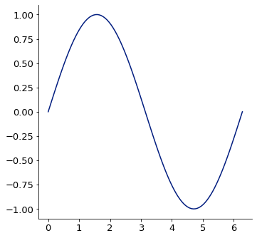
Regular matplotlib plotting syntax works:

import numpy as np
from McUtils.Plots import *

grid = np.linspace(0, 2*np.pi, 100)
plot = Plot(grid, np.sin(grid))
plot.show()

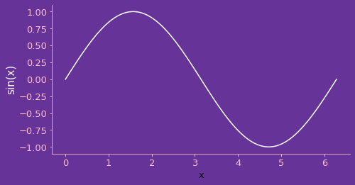
You can also set a background / axes labels / other options

plot = Plot(grid, np.sin(grid),
        plot_style={'color':'white'},
        axes_labels = ['x', Styled("sin(x)", color='white', fontsize=15)],
        frame_style={'color':'pink'},
        ticks_style={'color':'pink', 'labelcolor':'pink'},
        background = "rebeccapurple",
        image_size=500,
        aspect_ratio=.5
        )

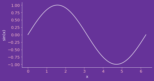
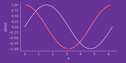
lots of styling can sometimes be easier to manage with the theme option, which uses matplotlib’s rcparams:

from cycler import cycler # installed with matplotlib

base_plot = Plot(grid, np.sin(grid),
        theme = ('mccoy', 
                 {
                     'figure.facecolor':'rebeccapurple',
                     'axes.facecolor':'rebeccapurple',
                     'axes.edgecolor':'white', 
                     'axes.prop_cycle': cycler(color=['white', 'pink', 'red']),
                     'axes.labelcolor':'white',
                     'xtick.color':'pink', 
                     'ytick.color':'pink'
                 }
                ),
        axes_labels = ['x', "sin(x)"],
        image_size=500,
        aspect_ratio=.5
        )

it’s worth noting that these styles are “sticky” when updating the figure

Plot(grid, np.cos(grid), figure=base_plot)

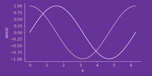
Plot(grid, np.cos(.1+grid), figure=base_plot)

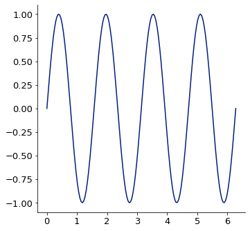
You can also plot a function over a given range

Plot(lambda x: np.sin(4*x), [0, 2*np.pi])

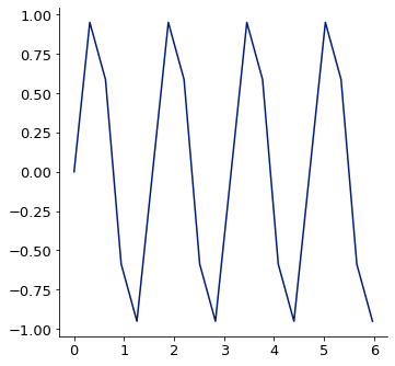
and you can also specify the step size for sampling the plotting range

Plot(lambda x: np.sin(4*x), [0, 2*np.pi, np.pi/10])

Edit Examples or Create New Examples
Edit Template or Create New Template
Edit Docstrings