Discrete Variable Representation
Discrete variable representation (DVR) is commonly used in the group and has quickly become a jumping off point for anyone getting started. Why? Because DVR is a simple way to dip your toes into challenging problems while the mechanics and math still stay relatively straight forward. (read as: “Easy to set up and great for exploring parameter space and gaining intuition”)
At its heart, DVR is about finding the “best” basis for representing operators that are functions of just our coordinates (i.e. that don’t involve things like derivatives of the wavefunction). To do this, we actually start with one of the bases we’ve talked about before, like the PIB, and build a representation for the coordinate operator.1 I.e. we set up the matrix
\[X_{i,j} = \langle i|\hat{x}|j \rangle\]then we make use of one of the fundamentals of our flavor of linear algebra, which is that diagonalization of an operator representation returns the best possible basis for that operator.
Why do we care about having the best basis for coordinate-only operators? Really just because the potential is this kind of operator and the potential is the hardest thing to deal with in a traditional basis set calculation. By choosing the best basis for the potential, we can dramatically decrease the amount of work we need to do. In fact, as we’ll see, for multiplicative operators like the potential, we won’t have to do any integrals at all.
Grid Points and the DVR Transformation
Diagonalization is something computers can do quickly and easily. In general it means finding matrices $Q$ and $X^D$ such that $X^D$ is diagonal and
\[X^D = Q^{-1}XQ\]We typically deal with Hermitian matrices for the systems that we approach where the matrix is self-adjoint, and so for everything we do we have the nice property that
\[Q^{T} = Q^{-1}\]therefore we’ll write
\[X^D = Q^{T}XQ\]$Q$ here is what we’ll call our DVR transformation. It takes operators represented in our original basis and transforms them to the DVR basis. How is the DVR basis the “best” basis for coordinate-only operators? Well $X^D$ is the representation of our coordinate operator in the basis defined by $Q$, and this representation is diagonal. We can’t really hope to do better than that.
These diagonal values are what we call our grid points or DVR points. It turns out that our DVR transformation does something very special, too. Calling our DVR basis functions $\phi_i^{\text{(DVR)}}$ and our grid points $x_i$, we get that
\[\phi_j^{\text{(DVR)}}(x) = f_i \delta_{i,j}\]where $f_i$ is just a normalization factor.
This means that these DVR functions are localized around their grid points and zero at all the others. That property will lead to some very useful results when setting up our Hamiltonian/using the resultant wavefunctions.
The DVR transformation allows us to switch smoothly between this discretized representation and the continuous representation from our original basis. Say we’ve got a simple representation for some operator $M$ in our original basis. We can do a change of basis to put this representation into the DVR basis by
\[M^{\text{(DVR)}} = Q^{T}MQ\]We can also go backwards by switching the order of multiplications. This allows us to reap the benefits of both representations, should that be something we find useful.
Colbert-Miller DVR (Particle in an Infinite Box)
One particular flavor of DVR that we like to use is the one described by Colbert and Miller in the early 1990s. There are three reasons we like this one:
- There are analytic forms for the kinetic energy
- The grid points are evenly spaced
- It’s appropriate for most non-periodic wavefunctions
Their approach actually differs from the one we detailed here, although the core idea is the same. The effect is to start with particle in a box basis functions, apply the type of DVR transformation that we describe here, then take the limit as the box and number of basis functions become infinite.
The end result of this is that their DVR basis functions are shifted $\frac{\sin(\theta)}{\theta}$ functions, which look like
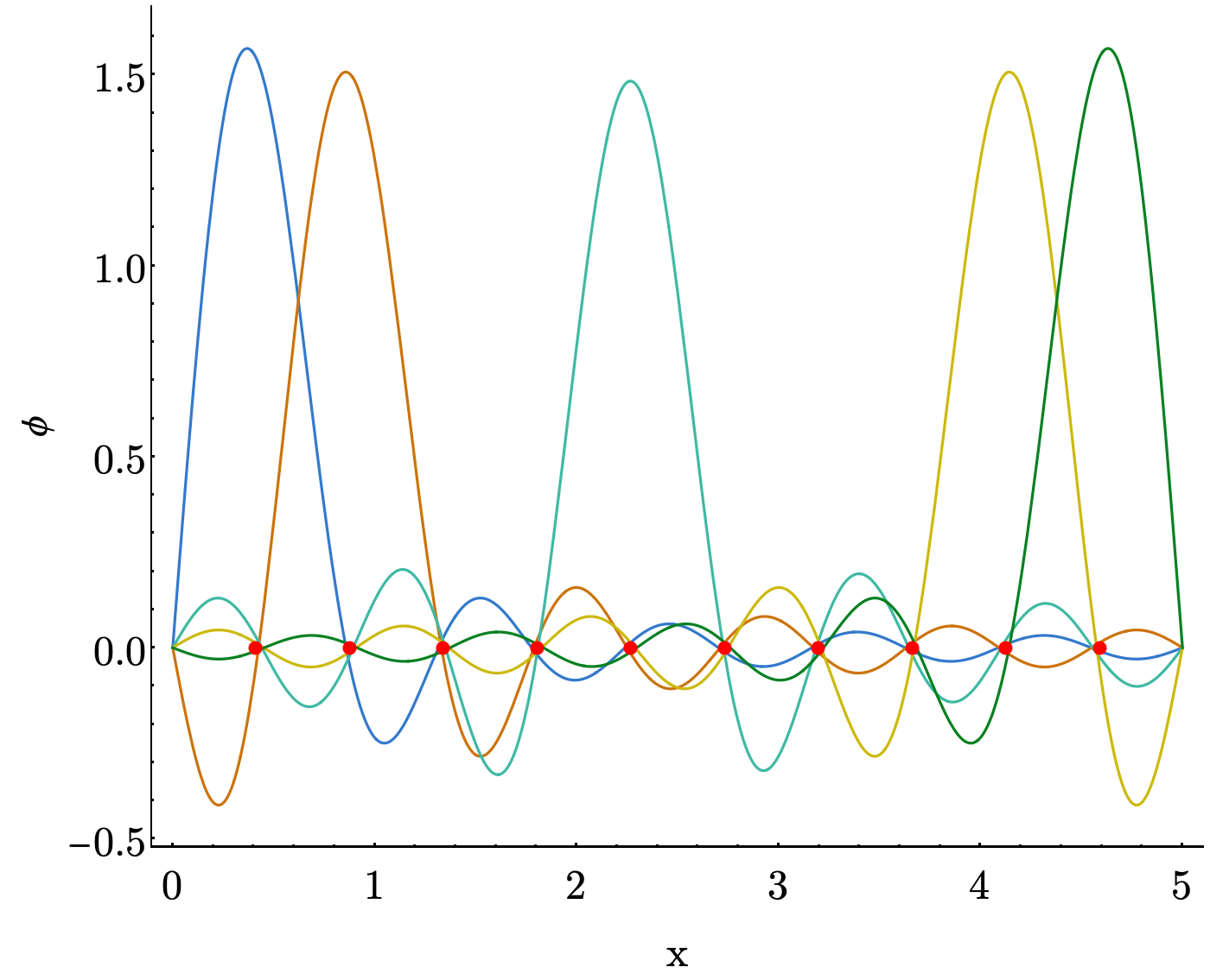
Note: In this graph we are only showing 5 of the basis functions, but if we were to keep plotting more we would see a peak at every discretized point.
We recommend looking at Appendix A of Colbert and Miller’s paper for the equations, starting with the (- $\infty$, $\infty$) interval! (i.e. your kinetic energy is described by Equation A7) But note you will need some potential function to run this all the way through. Seems like the perfect place for a harmonic oscillator!
Choice of Original Basis
The constraints of our problem strongly determine what types of bases are appropriate, which in turn determines what flavor of DVR we use. We’re not gonna get into every possible, reasonable choice, but ~1993 Szalay published a paper with a bunch of the different flavors worked out. For instance, in problems where we have an angle that can only range from $[0, \pi]$, the Legendre polynomials ($P_l$) are a good choice to satisfy that condition. They look like
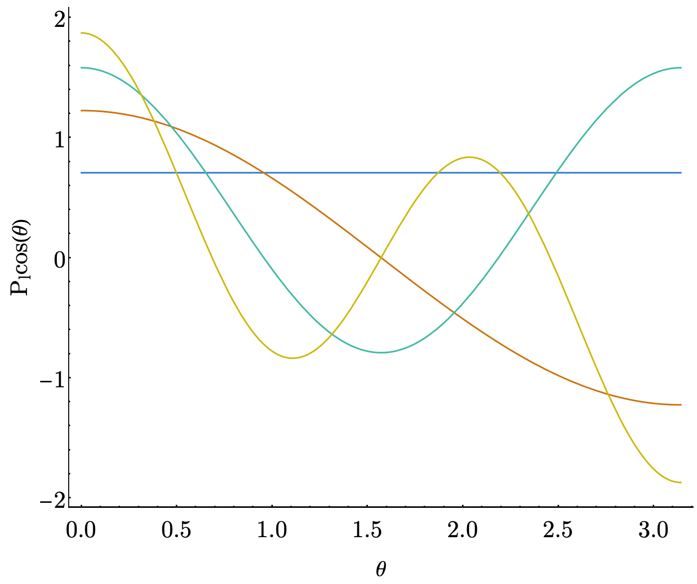
We play an interesting trick, here, where instead of using $\hat{x}$ as our coordinate operator, we use $cos(\theta)$ instead. This greatly simplifies the problem of evaluating the coordinate matrix elements. We also need to account for an extra “volume element” in our integrals, i.e. our coordinate operator matrix looks like
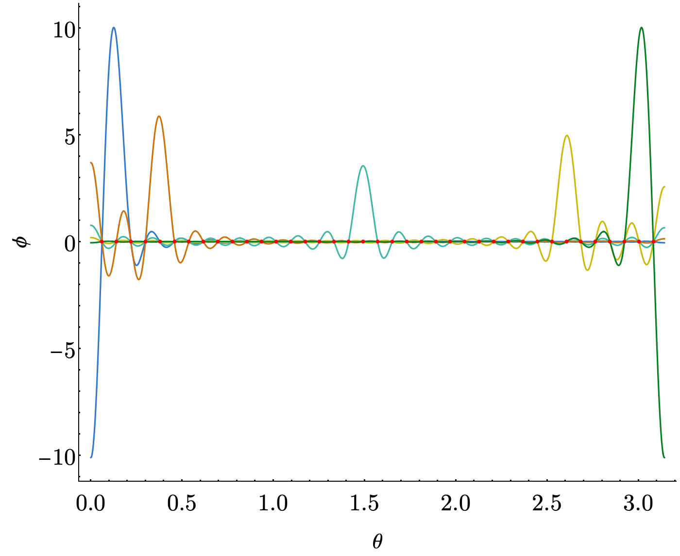
\[X_{i,j}=\langle i|\cos(\theta)|j\rangle= \int_{0}^{\pi} P_i(\cos(\theta))\cos(\theta)P_j(\cos(\theta))\sin(\theta) d \theta\]Once we do this, we get a clean representation as
\[X_{i,j} = \begin{cases} \sqrt{\frac{i^2}{(2 i + 1)(2 i - 1)}} & j = i+1 \\ \sqrt{\frac{j^2}{(2 j + 1)(2 j - 1)}} & i = j+1 \\ 0 & \text{else} \end{cases}\]and our basis functions now look like
For periodic problems on a $[0, 2\pi]$ range, there are different types of DVRs out there, like this one by Meyer.
Evaluation of Properties
Just as for a representation in a more “traditional” basis, if we want to get the expected value of an observable, $\hat{O}$, between states $\phi_n$ and $\phi_m$, we have
\[\langle O\rangle_{n,m} = c^{n}\textbf{O}c^{m}\]where $\textbf{O}$ is the matrix representation of $\hat{O}$ in our DVR basis and $c^{n}$ and $c^{m}$ are the coefficient vectors that come out of diagonalizing our Hamiltonian.
At this point, though, we’ll recall that for any multiplicative operator we have
\[\begin{align} \textbf{O}_{i,j} &= \left\langle \phi^{\text{DVR}}_i \lvert \hat{O} \rvert \phi^{\text{DVR}}_j \right\rangle \\ &= O(x_i) \delta_{i,j} \end{align}\]therefore assuming $\hat{O}$ is multiplicative (like the dipole moment or an internal coordinate) $\textbf{O}$ is diagonal, which means we can write
\[\begin{align} {\langle O \rangle}_{n,m} &= \sum_i O(x_i)c^{n}_{i}c^{m}_i \\ &= O(\textbf{x})\cdot(c^{n}c^{m}) \end{align}\]where $c^{n}c^{m}$ are multiplied element-wise. Computationally, this can be efficient, but even more than that this can be a nice conceptual way to think about these evaluation as we can build something akin to a probability density function for the transition by
\[\rho_{n,m} = \phi_{n}\phi_{m}\]and then in the point-wise representation $c^{n}c^{m}$ is this probability density.
If that does nothing for you conceptually, that’s cool too. Algorithmically it’s still a convenient way to write things.
Sample Applications
There are tons of applications for DVR out there. It’s one of the main tools that we keep in our toolbox. To get you started, we’ve got an exercise on writing your first Colbert & Miller-style DVR. Check it out.
Explore the Parameter Space
Once you have your DVR implementation up and running, play around and explore the parameter space! Some suggestions:
- Your two parameters in the DVR are the domain your gridpoints are on, and the number of grid points you have. So, what happens when you try say 200 gridpoints? 500? 2000? What about 50? or maybe even 10? As for the domain, what is effected (energies, wavefunction shape, both, neither) when you double the domain? quadruple it? divide it by 2? This is a good place to get started thinking about things like wavefunction convergence and numerical stability.
- What other simple diatomics can you look at? You can use the NIST Webbook and pull Constants of Diatomic Molecules for most diatomics and calculate the energies.
- What is the really difference between a Morse Oscillator and a Harmonic Oscillator? For one diatomic, say HCl, how much do the energies change? Why do you think that is?
- How much do the two models (Harmonic and Morse Oscillator) differ from the potential given by an electronic structure calculation? Why? Do the energies change? By how much? Which states seem to be affected by this the most (hint: think higher or lower energy states).
A Note on Parameters from the NIST Webbook
While the Constants of Diatomic Molecules Table may seem large and daunting at first hopefully keeping these hints in mind will help!
- The data you’re after is listed as the $X^1$ state (look for the ground electronic state)
- While the table has parameters $D_e$ and $\alpha_e$ these are not equivalent to the parameters $D_e$ and $\alpha$ of the Morse Oscillator. It goes something like “These aren’t the droids you are looking for…” right?
- INSTEAD, you will need to derive the values of $D_e$ and $\alpha$ from the parameters $\omega_e$ and $\omega_ex_e$.
As you do this, you’ll need to wrangle everyone’s favorite thing: units So, take this as a “right of passage” and work out how to solve for these parameters on your own. It takes some algebra and a good think about what the units need to be to make the answer have the correct units. If you’d like some advice on where to start, ask a group member.
Here’s a bit of necessary background info. Using a Taylor expansion we have
\[V(r_e) = \alpha^2D_e\Delta r^2 - \alpha^3D_e\Delta r^3 + \frac{7}{12}\alpha^4D_e\Delta r^4 + O(\Delta r^5)\]and so
\[\begin{align} \omega_e &= \sqrt{\frac{1}{\mu} \frac{\partial^2V}{\partial r^2} (r_e)} \\ \omega_ex_e &= -\frac{1}{16 \mu^2\omega_e^2} \left( F_4 - \frac{5}{3} \frac{ {F_3}^2 }{F_2} \right) \\ F_N &= \frac{\partial^{N} V}{\partial r^N} (r_e) \end{align}\]Got questions? Ask them on the McCoy Group Stack Overflow