Basic Diffusion Monte Carlo
Brief Overview of the Theory
As is shown in Anderson et. al. and is discussed in Suhm and Watts, the ground state solution to the time-independent Schrodinger Equation is solved using the time-dependent Schrodinger Equation. To begin, a variable substitution takes place (known as a Wick rotation) into imaginary time ($\tau=it/\hbar$). The energy is then shifted by some reference energy. We then propagate the wave function forward in time using discrete time steps:
\[\Psi(x, \tau + \Delta\tau) = e^{-(\hat{H}\Delta\tau})\Psi(x, \tau)\] \[\Psi(x, \tau + \Delta\tau) \approx e^{-(\hat{V} - E_{ref})\Delta\tau}e^{-\hat{T}\Delta\tau}\Psi(x, \tau)\]We approximate the time evolution operator by splitting it into exponential kinetic and potential energy operators. When we operate with the exponential kinetic and potential energy operator, we have stepped forward in time! The time-dependent wave function can always be written as a linear combination of eigenstates of the Hamiltonian multiplied by a time-dependent part like the following:
\[\Psi(x, \tau) = \sum_n c_{n}\psi_n(x)e^{-(E_n-E_{ref}(\tau))\tau}\]In the long time limit, the exponent becomes a large negative number, causing most terms to go to 0. The ground state will decay the slowest. This exponential decay can be seen in the following figure for different values of Eref.
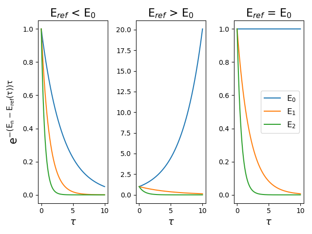
We see that when Eref is less than E0, all states decay to zero, but the ground state decays the slowest. When Eref is greater than E0, the contribution of the ground state dominates. During the course of the simulation, when the amplitude of the ground state becomes constant, Eref = E0, and the n=0 term’s exponential goes to 1 (as the exponent will go to 0) meaning that at long τ we will get the ground state solution! :)
The Algorithm
Now let’s talk about how we can actually implement this to obtain our ground state solution. On a simple level, this algorithm boils down to four steps.
- Displace the coordinates of your walkers
- Calculate the potential energy of your walkers
- Birth and death of the walkers
- Calculate Eref
These steps are repeated until the end of the simulation. The exception is for the first step where the Eref has not been calculated yet, which is essential in the birth and death step. So, for the first step, what is usually done is the potential energy of the walkers is calculated, followed by a calculation of Eref, then the four steps are looped until the end of the simulation.
So, for the first step where we displace the coordinates, this comes from the action of the kinetic energy operator operating on our wave function. This is a good exercise that will left to the reader where the result of operating on our localized function is that we get a gaussian distribution with width equal to (Δτ/m)1/2 where m is the mass associated with our system (all in atomic units). If we were modeling an OH stretch, the mass would be the reduced mass. How this plays out algorithmically is that we will displace our walkers randomly according to this Gaussian distribution. This can be shown in the following figure:
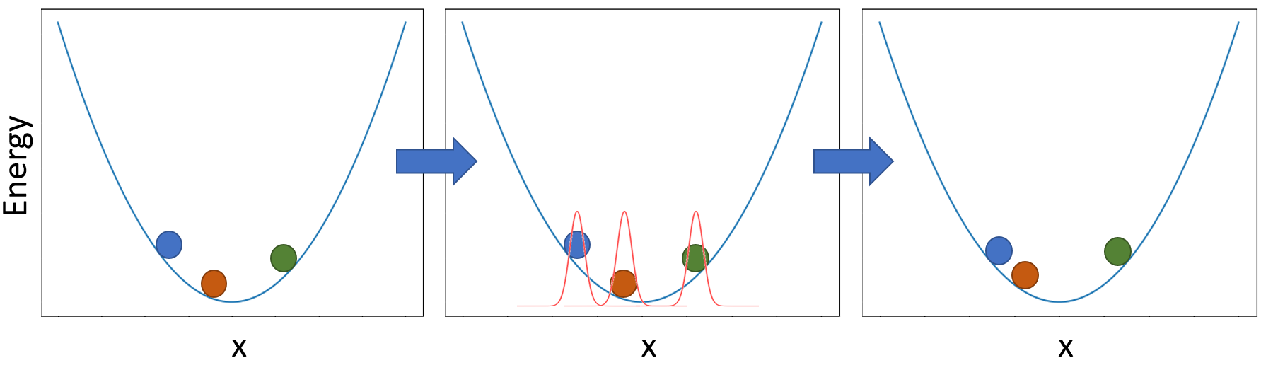
In the first panel we have a set of three walkers on our potential energy surface. Then according to the gaussian distribution discussed above, the walkers are moved randomly in the second and third panel.
The next step is using those displaced coordinates to evaluate the potential energy for each of our walkers in the ensemble. The potential depends on our system and is a function you will be providing the simulation. The example above is a simple harmonic oscillator.
The third step we are comparing the potential energy of our walkers to the value of Eref from the previous step. This is to check the favorability of its ‘random walk’, for example, if it moved into a classically forbidden region of the potential (higher energy) or classically allowed region (lower energy). If the energy is larger than Eref, there is a probability that this walker will be removed from the simulation (lab speak: “death”). If the energy is lower than this value, there is a probability that this walker will spawn replicates (lab speak: “birth”) into our simulation. To do this, we calculate the following exponential for each walker:
\[e^{-(V(x_j)-E_{ref})\Delta\tau}\]Following the procedure outlined in Anne’s paper here, for each walker we will take the integer value of this exponential and make that many clones into a new array. Then the fractional part is taken as a probability to create one extra copy of that walker. For example, if this exponential value for one walker is 4.7, 4 identical copies of that walker get put into the new array and that is a 70% chance for a fifth. If this exponential is 0.4, then there is only a 40% chance that the walker will stick around. This can be shown in the following figure:
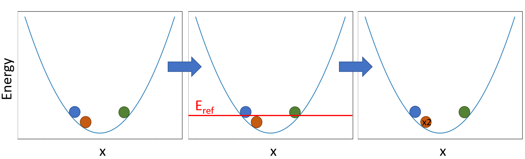
We see that the walkers are compared to the value of Eref for this set of walkers. Since the orange walker was below Eref, it had a chance to make a clone of itself and it did, yielding a total of two orange walkers for the next step in the simulation.
The last step is calculating Eref. This is done with the following equation:
\[E_{ref}(\tau) = \bar{V}(\tau) - \alpha \frac{N(\tau) - N(\tau_0)}{N(\tau_0)}\]Where the first term is the average potential energy of our ensemble at this time step, and the second term ensure that the number of walkers remain roughly constant. That α term is usually set equal to 1/(2Δτ) and the N is equal to the number of walkers.
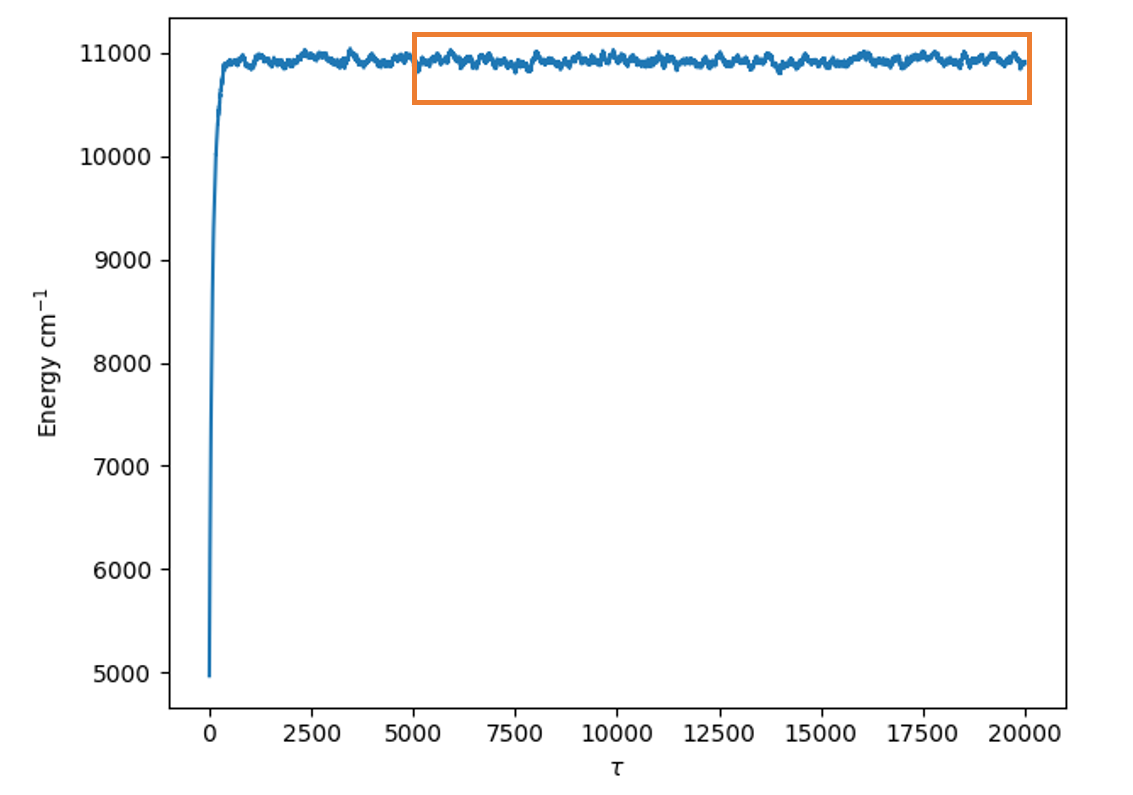
All of this is then repeated until the end of the simulation where you end up with an array of Eref values as a function of time step. To obtain the zero point energy for the system, we will take an time average of Eref from an equilibrated point in our simulation until the end of the simulation. A safe bet for “equilibrated” is half way through the simulation, but many times we will go to earlier values of time as well. This averaged value should not fluctuate much depending on when you decide to start averaging. An example of the section typically averaged to calculate the zero-point energy is shown in the following figure:
Differences Between Discrete and Continuous Weighting
The biggest difference between these two types of simulations is that discrete weighting has a fluctuating population where the weight of each walker is 1, while in continuous weighting the population is held constant while the weight of each walker is allowed to fluctuate. How this works in our algorithm is that for the birth and death step, the probability for a walker’s birth and death becomes equal to the weight that walker contributes to the total ensemble. This means that instead of a walker replicating itself when it is in favorable regions of the potential, the weight of the walker increases. One consequence with this method is that a walker could stay in a favorable region of the potential and have a weight so large that it dominates the ensemble. In order to mitigate this, we replace walkers whose weight falls below a certain threshold with a replicate of the highest weight walker. Then, the two walkers’ weights are cut in half.
The second difference is that Eref is calculated using the sum of the weights of the walkers instead of the number of walkers. This is technically the same equation since in the discrete weighting case, the weight of each walker is 1, so the sum of the weights of the walkers is equal to the number of walkers.
Got questions? Ask them on the McCoy Group Stack Overflow