Descendant Weighting and Wave Function Analysis
What is Descendant Weighting
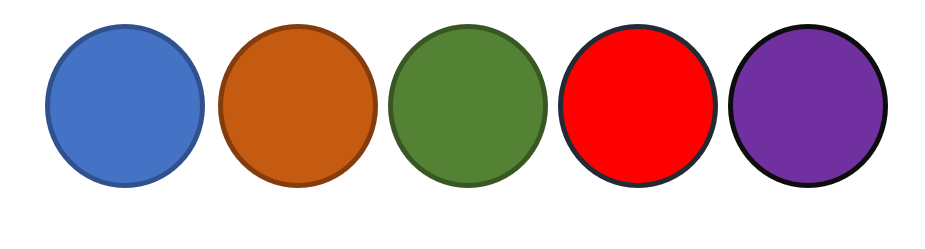
We’ve gone over how to run a basic DMC simulation but now what should we do with these walkers? Well, we have a wave function, but the important and interesting part having this is really $\Psi^{2}$. Since in DMC the representation of the wave function is (1) full-dimensional and (2) an ensemble of localized functions, we need to (1) project the wave function down to one or two dimensions to understand the probability amplitude and (2) use a technique to transform our ensemble data into (what appears to be) a continuous function. To accomplish this task we will use a technique called descendant weighting. This technique has been described by Suhm and Watts, and it boils down to keeping track of the descendants of each walker over a certain time. To be more specific, say we have a snapshot of our walkers at time $\tau$, then we want to track the descendants of those walkers until some time $\tau$’. So, for example lets say we have the following set of walkers at time $\tau$.
Then we will track the descendants of these walkers over a set amount of time. For example, the following figure shows how the walkers propogate over 5 time steps.
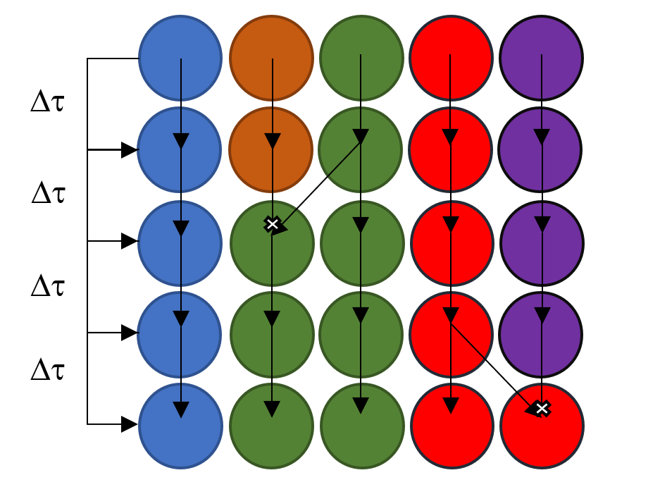
We see that the orange walker dies after 2 time steps and the green walker gives birth. Then after four time steps the purple walker dies and a red one gives birth. For discrete weighting you would just count up the number of walkers that each walker produced at the end. For example, the green walker would have a descendant weight of 2, while the purple walker would have a descendant weight of 0. For continuous weighting, you would add up the weight of each walker’s descendants. For example, let’s say that the two green walkers at the end had weights of 1.2 and 0.9, then the descendant weight of the green walker would be 2.1. The number of time steps allows for the ensemble to propagate is not an exact science; there is an interplay between the two edge cases, where if one propagates for too few steps the wave function will not have changed enough for it to be another true representation of $\Psi$, if one propagates for too long the walkers at time $\tau$ may collapse onto too few walkers, making both the accuracy and the precision of $\Psi^2$ incorrect. You may want to play around with this to get an intuition for it!
Using Descendant Weights
Now that we have these descendant weights, we can obtain a projection of the probability amplitude onto some desired coordinate of interest through a histogram. The histogram effectively smoothes our data into a pseudo-continuous function. If we were projecting $\Psi^2$ onto a bond length (say the OH stretch of water), we will calculate that bond length for each walker, and then assign each walker into a segment along a discretized, paritioned x-axis (called a “bin” in histogram language). The amplitude (y-axis) contribution of each walker is its descendant weight. This yields the probability amplitude along the coordinate!
[Example Histogram]
Additionally, if we wanted an expectation value (integral) of a specific operator then all we have to do is use a method called Monte Carlo Integration:
\[\langle A\rangle = \frac{\sum_j d_j A_j}{\sum_j d_j}\]Where $A_j$ is any multiplicative operator (potential energy, displacement, dipole moment, etc.) of interest and $d_j$ is the descendant weight of the $j$th walker. Each walker will have a different value of $A$.
Got questions? Ask them on the McCoy Group Stack Overflow