Stick Spectra
When an experimentalist collects an infrared/vibrational spectrum, the signal they tend to get out generally looks something like this1
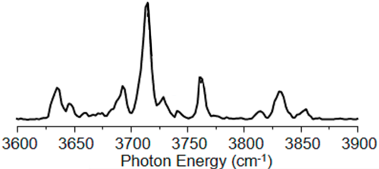
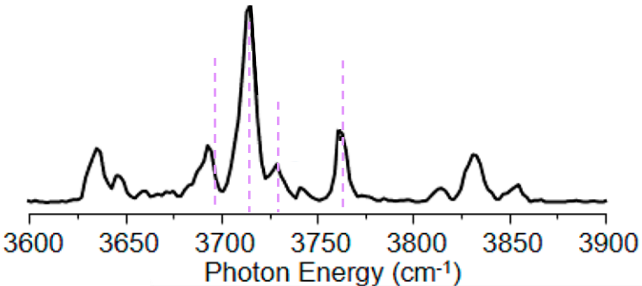
We can see that there are well defined peaks or “features”, which have a maximum at a given frequency, but these features also have a width to them. That width is a time-dependent, dynamical effect and goes beyond what we as a group generally are interested in. So when we calculate a spectrum, we usually calculate a stick spectrum, which is a set of frequencies and associated intensities, that can be plotted like
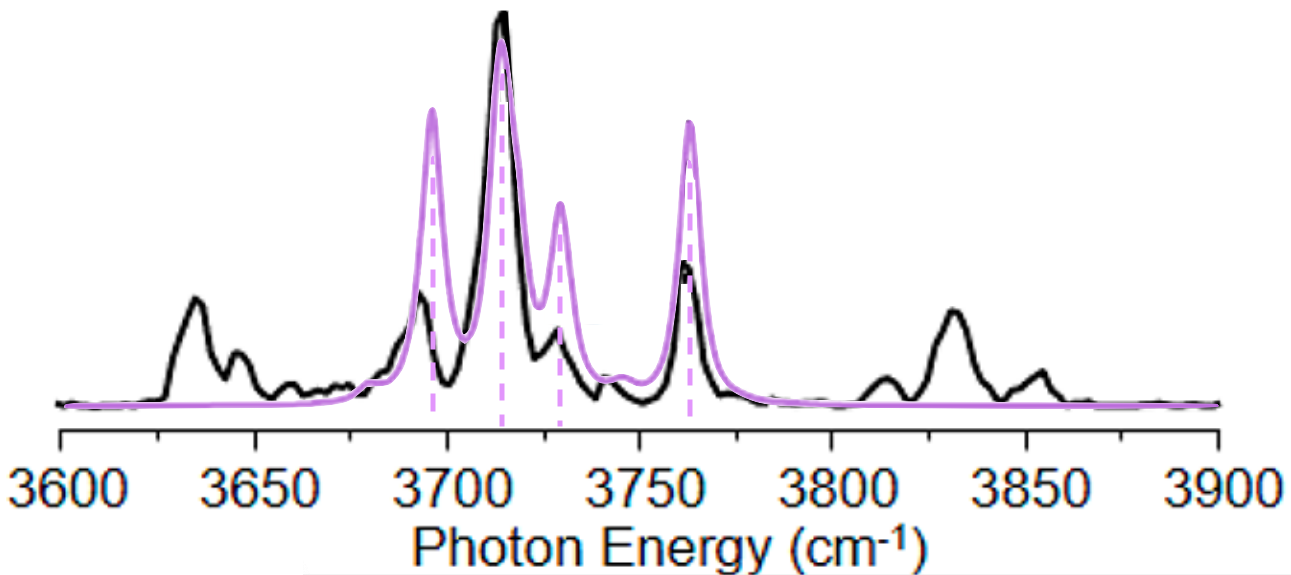
and then to make comparisons to experiment a bit cleaner, we’ll choose a width, or amount of broadening, and multiply each intensity by a normal distribution with that width centered around its associated frequency. You will often hear this described as “convolving with a Gaussian”.
At the end of the day, that means we end up with a spectrum that looks like
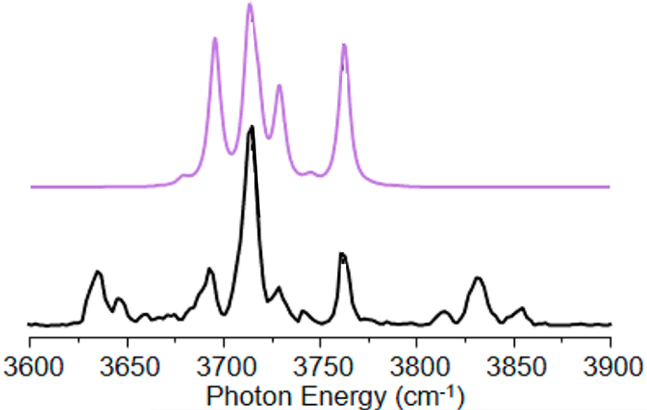
or a bit cleaner for the purposes of comparison
A Note on Units
Recalling from the overview that we get our stick spectra from
\[I_{n,m} \propto \nu_{n,m} {\left\lvert \left\langle \psi_n | \mu | \psi_m \right\rangle \right\rvert}^{2}\]We see that we only have a proportionality. Given that many experimental intensities are reported in “arbitrary” units, that’s okay, since we can simply normalize our stick spectrum to some peak in the experimental one.
On the other hand, there are cases where we do care about units, especially when comparing between different methods for calculating spectra. In that case, we generally have three equivalent units we can report things in. The first is the oscillator strength, which is essentially the ratio between the intensity that would be predicted quantum mechanically for the transition vs. classically for a single electron oscillating in 3D (i.e. an early model of the hydrogen atom). This is given by2
\[f_{n m} = \frac{4 \pi m_e}{3 e^2 \hbar} \nu_{n,m} {\left\lvert \left\langle \psi_n | \mu | \psi_m \right\rangle \right\rvert}^{2}\]where $m_e$ is the mass of the electron and $e$ is the elementary charge. This is commonly re-expressed in units that people actually use, i.e. wavenumbers & Debye, to give
\[f_{n m} = 4.70165 \times 10^{-7} (\text{cm}\ \text{D}^{-2}) \times \nu_{n,m} {\left\lvert \left\langle \psi_n | \mu | \psi_m \right\rangle \right\rvert}^{2}\]The second unit people care about is are $\text{km}\ \text{mol}^{-1}$. These are essentially the gas-phase appropriate units for the $\varepsilon$ in Beer’s Law
\[A = \varepsilon l c\]This is also called the absorption coefficient. Happily, it’s straight-forward to convert from oscillator strengths to these units, by3
\[\varepsilon_{n m} = 5.33049 \times 10^6 (\text{km}\ \text{mol}^{-1}) \times f_{n m}\]Finally, experimentalists also report absorptions in terms of the integrated cross section, $\sigma$, which is essentially the interaction probability normalized by the number of particles. The units we like for this are $\text{cm}\ \text{molecule}^{-1}$ and can be gotten from the oscillator strength by3
\[\sigma_{n m} = 8.85 \times 10^{-13} (\text{cm}\ \text{molecule}^{-1}) \times f_{n m}\]Got questions? Ask them on the McCoy Group Stack Overflow
- https://doi.org/10.1021/acs.jpca.0c00853
- https://doi.org/10.1063/1.458993 or Atkins’ Molecular Quantum Mechanics
- https://doi.org/10.1063/1.458993 or https://doi.org/10.1063/1.4921731