McUtils
A growing package of assorted functionality that finds use across many different packages, but doesn’t attempt to provide a single unified interface for doing certain types of projects.
All of the McUtils packages stand mostly on their own, but there will be little calls into one another here and there,
especially pieces using Numputils
The more scientifically-focused Psience package makes significant use of McUtils as do various packages that have
been written over the years.
Members
Examples
We will provide a brief examples for the common use cases for each module. More information can be found on the pages themselves. The unit tests for each package are provided on the bottom of the package page. These provide useful usage examples.
Parsers
The Parsers package provides a toolkit for easily parsing string data out of files.
Here we’ll get every key-value pair matching the pattern key = value from a Gaussian .log file
test_data = os.path.join(os.path.dirname(McUtils.__file__), 'ci', 'tests', 'TestData')
with open(os.path.join(test_data, 'water_OH_scan.log')) as log_dat:
    sample_data = log_dat.read()

key_value_matcher = RegexPattern([Named(Word, "key"), "=", Named(Word, "value")])
key_vals = StringParser(key_value_matcher).parse_all(sample_data)
key_vals['key'].array
array(['0', 'Input', 'Output', ..., 'State', 'RMSD', 'PG'], dtype='<U7')
It’s used extensively in the GaussianInterface package.
Plots
A layer on matplotlib to provide more declarative syntax and easier composability.
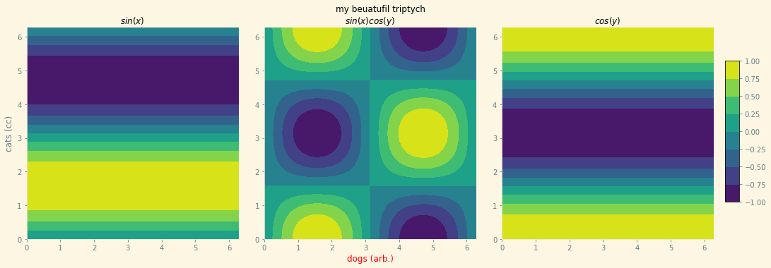
Here we’ll make a styled GraphicsGrid
grid = np.linspace(0, 2 * np.pi, 100)
grid_2D = np.meshgrid(grid, grid)
x = grid_2D[1]
y = grid_2D[0]

main = GraphicsGrid(ncols=3, nrows=1,
                    theme='Solarize_Light2', figure_label='my beuatufil triptych',
                    padding=((35, 60), (35, 40)), subimage_size=300)
main[0, 0] = ContourPlot(x, y, np.sin(y), plot_label='$sin(x)$',
                         axes_labels=[None, "cats (cc)"],
                         figure=main[0, 0]
                         )
main[0, 1] = ContourPlot(x, y, np.sin(x) * np.cos(y),
                         plot_label='$sin(x)cos(y)$',
                         axes_labels=[Styled("dogs (arb.)", {'color': 'red'}), None],
                         figure=main[0, 1])
main[0, 2] = ContourPlot(x, y, np.cos(y), plot_label='$cos(y)$', figure=main[0, 2])
main.colorbar = {"graphics": main[0, 1].graphics}
Data
Provides access to relevant atomic/units data pulled from NIST databases.
Pull the record for deuterium
AtomData["D"]
DataRecord('D', AtomDataHandler('AtomData', file='None'))
Grab the isotopically correct atomic mass
AtomData["D", "Mass"]
2.01410177812
Get all possible keys
AtomData["D"].keys()
dict_keys(['Name', 'Symbol', 'Mass', 'Number', 'MassNumber', 'IsotopeFraction', 'CanonicalName', 'CanonicalSymbol', 'ElementName', 'ElementSymbol', 'IconColor', 'IconRadius', 'PrimaryIsotope', 'StandardAtomicWeights'])
Get the conversion from Hartrees to wavenumbers
UnitsData.convert("Hartrees", "Wavenumbers")
219474.6313632
This conversion is not in the underlying database but is computed implicitly. Another example
UnitsData.data[("AtomicMassUnits", "Wavenumbers")]
KeyError: ('AtomicMassUnits', 'Wavenumbers')
UnitsData.convert("AtomicMassUnits", "Wavenumbers")
7513006610400.0
UnitsData.data[("AtomicMassUnits", "Hartrees")]
{'Value': 34231776.874,
 'Uncertainty': 0.01,
 'Conversion': ('AtomicMassUnits', 'Hartrees')}
Coordinerds
Provides utilities for writing coordinate conversions and obtaining Jacobians between coordinate systems. First we make a set of Cartesian coordinates
struct = [
            [ 0.0,                    0.0,                   0.0                ],
            [ 0.5312106220949451,     0.0,                   0.0                ],
            [ 5.4908987527698905e-2,  0.5746865893353914,    0.0                ],
            [-6.188515885294378e-2,  -2.4189926062338385e-2, 0.4721688095375285 ],
            [ 1.53308938205413e-2,    0.3833690190410768,    0.23086294551212294],
            [ 0.1310095622893345,     0.30435650497612,      0.5316931774973834 ]
        ]
coords = CoordinateSet(struct)
CoordinateSet([[ 0.        ,  0.        ,  0.        ],
               [ 0.53121062,  0.        ,  0.        ],
               [ 0.05490899,  0.57468659,  0.        ],
               [-0.06188516, -0.02418993,  0.47216881],
               [ 0.01533089,  0.38336902,  0.23086295],
               [ 0.13100956,  0.3043565 ,  0.53169318]])
then convert that to Z-matrix coordinates
icrds = coords.convert(ZMatrixCoordinates)
CoordinateSet([[ 0.53121062,  0.        ,  0.        ],
               [ 0.74641002,  0.878738  ,  0.        ],
               [ 0.77151626,  1.04598737, -0.7854913 ],
               [ 0.47989075,  0.13178784, -2.07064742],
               [ 0.3318484 ,  0.92484778,  2.60361273]])
we can also get the Jacobian for the transformation
icrds = coords.convert(ZMatrixCoordinates)
array([[[[ -1.        ,   0.        ,   0.        ],
         [  0.        ,  -0.        ,   0.        ],
         [  0.        ,   0.        ,   0.        ],
         [  0.        ,   0.        ,   0.        ],
         [  0.        ,   0.        ,   0.        ]],

        [[  0.        ,   0.        ,   0.        ],
         [  0.        ,  -1.88249248,   0.        ],
         [  0.        ,   0.        ,   0.        ],
         [  0.        ,   0.        ,   0.        ],
         [  0.        ,   0.        ,   0.        ]],

        ...

        [[  0.        ,   0.        ,   0.        ],
         [  0.        ,   0.        ,   0.        ],
         [  0.61200111,   0.45926084,  -1.05894329],
         [  0.502835  ,  -0.77583777,  -0.70022831],
         [  0.        ,  -1.57576683,  -0.82116186]]],


       ...

        [[  0.        ,   0.        ,   0.        ],
         [  0.        ,   0.        ,   0.        ],
         [  0.        ,   0.        ,   0.        ],
         [  0.        ,   0.        ,   0.        ],
         [ -0.23809822,   2.66405562,   1.5176851 ]],

        [[  0.        ,   0.        ,   0.        ],
         [  0.        ,   0.        ,   0.        ],
         [  0.        ,   0.        ,   0.        ],
         [  0.        ,   0.        ,   0.        ],
         [  0.9065291 ,   0.16172563,   1.58012353]]]])
Zachary
Zachary is a higher-level package than Numputils and handles all numerical/tensor operations.
It’s become something of a monster but is very useful.
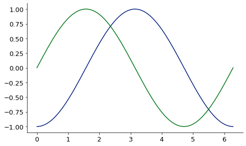
1D finite difference derivative via finite_difference:
from McUtils.Zachary import finite_difference
import numpy as np

sin_grid = np.linspace(0, 2*np.pi, 200)
sin_vals = np.sin(sin_grid)

deriv = finite_difference(sin_grid, sin_vals, 3) # 3rd deriv
base = Plot(sin_grid, deriv, aspect_ratio = .6, image_size=500)
Plot(sin_grid, np.sin(sin_grid), figure=base)
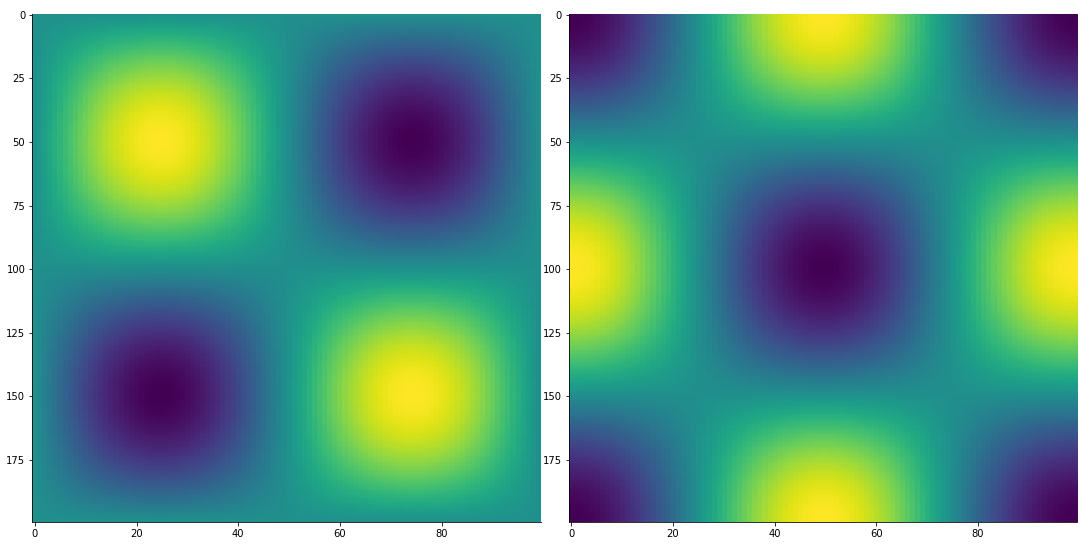
2D finite difference derivative via finite_difference:
from McUtils.Zachary import finite_difference
import numpy as np

x_grid = np.linspace(0, 2*np.pi, 200)
y_grid = np.linspace(0, 2*np.pi, 100)
sin_x_vals = np.sin(x_grid); sin_y_vals =  np.sin(y_grid)
vals_2D = np.outer(sin_x_vals, sin_y_vals)
grid_2D = np.array(np.meshgrid(x_grid, y_grid)).T

deriv = finite_difference(grid_2D, vals_2D, (1, 3))
TensorPlot(np.array([vals_2D, deriv]), image_size=500)
Also supported: Mesh operations, automatic differentiation, tensor derivative coordinate transformations, and Taylor series expansions of functions